Note
Access to this page requires authorization. You can try signing in or changing directories.
Access to this page requires authorization. You can try changing directories.
Switch services using the Version drop-down list. Learn more about navigation.
Applies to: ✅ Azure Data Explorer ✅ Azure Monitor ✅ Microsoft Sentinel
Graph semantics supports two primary approaches for working with graphs: transient graphs created in-memory for each query, and persistent graphs defined as graph models and snapshots within the database. This article provides best practices for both methods, enabling you to select the optimal approach and use KQL graph semantics efficiently.
This guidance covers:
- Graph creation and optimization strategies
- Querying techniques and performance considerations
- Schema design for persistent graphs
- Integration with other KQL features
- Common pitfalls to avoid
Graph modeling approaches
There are two approaches for working with graphs: transient and persistent.
Transient graphs
Created dynamically using the make-graph operator. These graphs exist only during query execution and are optimal for ad-hoc or exploratory analysis on small to medium datasets.
Persistent graphs
Defined using graph models and graph snapshots. These graphs are stored in the database, support schema and versioning, and are optimized for repeated, large-scale, or collaborative analysis.
Best practices for transient graphs
Transient graphs, created in-memory using the make-graph operator, are ideal for ad hoc analysis, prototyping, and scenarios where graph structure changes frequently or requires only a subset of available data.
Optimize graph size for performance
The make-graph creates an in-memory representation including both structure and properties. Optimize performance by:
- Apply filters early - Select only relevant nodes, edges, and properties before graph creation
- Use projections - Remove unnecessary columns to minimize memory consumption
- Apply aggregations - Summarize data where appropriate to reduce graph complexity
Example: Reducing graph size through filtering and projection
In this scenario, Bob changed managers from Alice to Eve. To view only the latest organizational state while minimizing graph size:
let allEmployees = datatable(organization: string, name:string, age:long)
[
  "R&D", "Alice", 32,
  "R&D","Bob", 31,
  "R&D","Eve", 27,
  "R&D","Mallory", 29,
  "Marketing", "Alex", 35
];
let allReports = datatable(employee:string, manager:string, modificationDate: datetime)
[
  "Bob", "Alice", datetime(2022-05-23),
  "Bob", "Eve", datetime(2023-01-01),
  "Eve", "Mallory", datetime(2022-05-23),
  "Alice", "Dave", datetime(2022-05-23)
];
let filteredEmployees =
    allEmployees
    | where organization == "R&D"
    | project-away age, organization;
let filteredReports =
    allReports
    | summarize arg_max(modificationDate, *) by employee
    | project-away modificationDate;
filteredReports
| make-graph employee --> manager with filteredEmployees on name
| graph-match (employee)-[hasManager*2..5]-(manager)
  where employee.name == "Bob"
  project employee = employee.name, topManager = manager.name
Output:
| employee | topManager |
|---|---|
| Bob | Mallory |
Maintain current state with materialized views
The previous example showed how to obtain the last known state using summarize and arg_max. This operation can be compute-intensive, so consider using materialized views for improved performance.
Step 1: Create tables with versioning
Create tables with a versioning mechanism for graph time series:
.create table employees (organization: string, name:string, stateOfEmployment:string, properties:dynamic, modificationDate:datetime)

.create table reportsTo (employee:string, manager:string, modificationDate: datetime)
Step 2: Create materialized views
Use the arg_max aggregation function to determine the latest state:
.create materialized-view employees_MV on table employees
{
    employees
    | summarize arg_max(modificationDate, *) by name
}

.create materialized-view reportsTo_MV on table reportsTo
{
    reportsTo
    | summarize arg_max(modificationDate, *) by employee
}
Step 3: Create helper functions
Ensure only the materialized component is used and apply another filters:
.create function currentEmployees () {
    materialized_view('employees_MV')
    | where stateOfEmployment == "employed"
}

.create function reportsTo_lastKnownState () {
    materialized_view('reportsTo_MV')
    | project-away modificationDate
}
This approach provides faster queries, higher concurrency, and lower latency for current state analysis while preserving access to historical data.
let filteredEmployees =
    currentEmployees
    | where organization == "R&D"
    | project-away organization;
reportsTo_lastKnownState
| make-graph employee --> manager with filteredEmployees on name
| graph-match (employee)-[hasManager*2..5]-(manager)
  where employee.name == "Bob"
  project employee = employee.name, reportingPath = hasManager.manager
Implement graph time travel
Analyzing data based on historical graph states provides valuable temporal context. Implement this "time travel" capability by combining time filters with summarize and arg_max:
.create function graph_time_travel (interestingPointInTime:datetime ) {
    let filteredEmployees =
        employees
        | where modificationDate < interestingPointInTime
        | summarize arg_max(modificationDate, *) by name;
    let filteredReports =
        reportsTo
        | where modificationDate < interestingPointInTime
        | summarize arg_max(modificationDate, *) by employee
        | project-away modificationDate;
    filteredReports
    | make-graph employee --> manager with filteredEmployees on name
}
Usage example:
Query Bob's top manager based on June 2022 graph state:
graph_time_travel(datetime(2022-06-01))
| graph-match (employee)-[hasManager*2..5]-(manager)
  where employee.name == "Bob"
  project employee = employee.name, reportingPath = hasManager.manager
Output:
| employee | topManager |
|---|---|
| Bob | Dave |
Handle multiple node and edge types
When working with complex graphs containing multiple node types, use a canonical property graph model. Define nodes with attributes like nodeId (string), label (string), and properties (dynamic), while edges include source (string), destination (string), label (string), and properties (dynamic) fields.
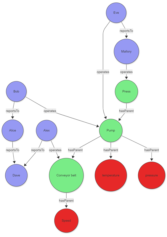
Example: Factory maintenance analysis
Consider a factory manager investigating equipment issues and responsible personnel. The scenario combines asset graphs of production equipment with maintenance staff hierarchy:
The data for those entities can be stored directly in your cluster or acquired using query federation to a different service. To illustrate the example, the following tabular data is created as part of the query:
let sensors = datatable(sensorId:string, tagName:string, unitOfMeasure:string)
[
  "1", "temperature", "°C",
  "2", "pressure", "Pa",
  "3", "speed", "m/s"
];
let timeseriesData = datatable(sensorId:string, timestamp:string, value:double, anomaly: bool )
[
    "1", datetime(2023-01-23 10:00:00), 32, false,
    "1", datetime(2023-01-24 10:00:00), 400, true,
    "3", datetime(2023-01-24 09:00:00), 9, false
];
let employees = datatable(name:string, age:long)
[
  "Alice", 32,
  "Bob", 31,
  "Eve", 27,
  "Mallory", 29,
  "Alex", 35,
  "Dave", 45
];
let allReports = datatable(employee:string, manager:string)
[
  "Bob", "Alice",
  "Alice", "Dave",
  "Eve", "Mallory",
  "Alex", "Dave"
];
let operates = datatable(employee:string, machine:string, timestamp:datetime)
[
  "Bob", "Pump", datetime(2023-01-23),
  "Eve", "Pump", datetime(2023-01-24),
  "Mallory", "Press", datetime(2023-01-24),
  "Alex", "Conveyor belt", datetime(2023-01-24),
];
let assetHierarchy = datatable(source:string, destination:string)
[
  "1", "Pump",
  "2", "Pump",
  "Pump", "Press",
  "3", "Conveyor belt"
];
The employees, sensors, and other entities and relationships don't share a canonical data model. The union operator can be used to combine and standardize the data.
The following query joins the sensor data with the time series data to identify sensors with abnormal readings, then uses a projection to create a common model for the graph nodes.
let nodes =
    union
        (
            sensors
            | join kind=leftouter
            (
                timeseriesData
                | summarize hasAnomaly=max(anomaly) by sensorId
            ) on sensorId
            | project nodeId = sensorId, label = "tag", properties = pack_all(true)
        ),
        ( employees | project nodeId = name, label = "employee", properties = pack_all(true));
The edges are transformed in a similar manner.
let edges =
    union
        ( assetHierarchy | extend label = "hasParent" ),
        ( allReports | project source = employee, destination = manager, label = "reportsTo" ),
        ( operates | project source = employee, destination = machine, properties = pack_all(true), label = "operates" );
With the standardized nodes and edges data, you can create a graph using the make-graph operator
let graph = edges
| make-graph source --> destination with nodes on nodeId;
Once the graph is created, define the path pattern and project the required information. The pattern begins at a tag node, followed by a variable-length edge to an asset. That asset is operated by an operator who reports to a top manager via a variable-length edge called reportsTo. The constraints section of the graph-match operator, in this case the where clause, filters the tags to those with an anomaly that were operated on a specific day.
graph
| graph-match (tag)-[hasParent*1..5]->(asset)<-[operates]-(operator)-[reportsTo*1..5]->(topManager)
    where tag.label=="tag" and tobool(tag.properties.hasAnomaly) and
        startofday(todatetime(operates.properties.timestamp)) == datetime(2023-01-24)
        and topManager.label=="employee"
    project
        tagWithAnomaly = tostring(tag.properties.tagName),
        impactedAsset = asset.nodeId,
        operatorName = operator.nodeId,
        responsibleManager = tostring(topManager.nodeId)
Output
| tagWithAnomaly | impactedAsset | operatorName | responsibleManager |
|---|---|---|---|
| temperature | Pump | Eve | Mallory |
The projection in graph-match shows that the temperature sensor exhibited an anomaly on the specified day. The sensor was operated by Eve, who ultimately reports to Mallory. With this information, the factory manager can contact Eve and, if necessary, Mallory to better understand the anomaly.
Best practices for persistent graphs
Persistent graphs, defined using graph models, and graph snapshots, provide robust solutions for advanced graph analytics needs. These graphs excel in scenarios requiring repeated analysis of large, complex, or evolving data relationships, and facilitate collaboration by enabling teams to share standardized graph definitions and consistent analytical results. By persisting graph structures in the database, this approach significantly enhances performance for recurring queries and supports sophisticated versioning capabilities.
Use schema and definition for consistency and performance
A clear schema for your graph model is essential, as it specifies node and edge types along with their properties. This approach ensures data consistency and enables efficient querying. Utilize the Definition section to specify how nodes and edges are constructed from your tabular data through AddNodes and AddEdges steps.
Use static and dynamic labels for flexible modeling
When modeling your graph, you can utilize both static and dynamic labeling approaches for optimal flexibility. Static labels are ideal for well-defined node and edge types that rarely change—define these in the Schema section and reference them in the Labels array of your steps. For cases where node or edge types are determined by data values (for example, when the type is stored in a column), use dynamic labels by specifying a LabelsColumn in your step to assign labels at runtime. This approach is especially useful for graphs with heterogeneous or evolving schemas. Both mechanisms can be effectively combined—you can define a Labels array for static labels and also specify a LabelsColumn to incorporate labels from your data, providing maximum flexibility when modeling complex graphs with both fixed and data-driven categorization.
Example: Using dynamic labels for multiple node and edge types
The following example demonstrates an effective implementation of dynamic labels in a graph representing professional relationships. In this scenario, the graph contains people and companies as nodes, with employment relationships forming the edges between them. The flexibility of this model comes from determining node and edge types directly from columns in the source data, allowing the graph structure to adapt organically to the underlying information.
.create-or-alter graph_model ProfessionalNetwork ```
{
  "Schema": {
    "Nodes": {
      "Person": {"Name": "string", "Age": "long"},
      "Company": {"Name": "string", "Industry": "string"}
    },
    "Edges": {
      "WORKS_AT": {"StartDate": "datetime", "Position": "string"}
    }
  },
  "Definition": {
    "Steps": [
      {
        "Kind": "AddNodes",
        "Query": "Employees | project Id, Name, Age, NodeType",
        "NodeIdColumn": "Id",
        "Labels": ["Person"],
        "LabelsColumn": "NodeType"
      },
      {
        "Kind": "AddEdges",
        "Query": "EmploymentRecords | project EmployeeId, CompanyId, StartDate, Position, RelationType",
        "SourceColumn": "EmployeeId",
        "TargetColumn": "CompanyId",
        "Labels": ["WORKS_AT"],
        "LabelsColumn": "RelationType"
      }
    ]
  }
}
```
This dynamic labeling approach provides exceptional flexibility when modeling graphs with numerous node and edge types, eliminating the need to modify your schema each time a new entity type appears in your data. By decoupling the logical model from the physical implementation, your graph can continuously evolve to represent new relationships without requiring structural changes to the underlying schema.
Multitenant partitioning strategies for large-scale ISV scenarios
In large organizations, particularly ISV scenarios, graphs can consist of multiple billions of nodes and edges. This scale presents unique challenges that require strategic partitioning approaches to maintain performance while managing costs and complexity.
Understanding the challenge
Large-scale multitenant environments often exhibit the following characteristics:
- Billions of nodes and edges - Enterprise-scale graphs that exceed traditional graph database capabilities
- Tenant size distribution - Typically follows a power law where 99.9% of tenants have small to medium graphs, while 0.1% have massive graphs
- Performance requirements - Need for both real-time analysis (current data) and historical analysis capabilities
- Cost considerations - Balance between infrastructure costs and analytical capabilities
Partitioning by natural boundaries
The most effective approach for managing large-scale graphs is partitioning by natural boundaries, typically tenant identifiers, or organizational units:
Key partitioning strategies:
- Tenant-based partitioning - Separate graphs by customer, organization, or business unit
- Geographic partitioning - Divide by region, country, or datacenter location
- Temporal partitioning - Separate by time periods for historical analysis
- Functional partitioning - Split by business domain or application area
Example: Multitenant organizational structure
// Partition employees and reports by tenant
let tenantEmployees =
    allEmployees
    | where tenantId == "tenant_123"
    | project-away tenantId;

let tenantReports =
    allReports
    | where tenantId == "tenant_123"
    | summarize arg_max(modificationDate, *) by employee
    | project-away modificationDate, tenantId;

tenantReports
| make-graph employee --> manager with tenantEmployees on name
| graph-match (employee)-[hasManager*1..5]-(manager)
  where employee.name == "Bob"
  project employee = employee.name, reportingChain = hasManager.manager
Hybrid approach: Transient vs. persistent graphs by tenant size
The most cost-effective strategy combines both transient and persistent graphs based on tenant characteristics:
Small to medium tenants (99.9% of tenants)
Use transient graphs for most tenants:
Advantages:
- Always up-to-date data - No snapshot maintenance required
- Lower operational overhead - No graph model or snapshot management
- Cost-effective - No extra storage costs for graph structures
- Immediate availability - No preprocessing delays
Implementation pattern:
.create function getTenantGraph(tenantId: string) {
    let tenantEmployees =
        employees
        | where tenant == tenantId and stateOfEmployment == "employed"
        | project-away tenant, stateOfEmployment;
    let tenantReports =
        reportsTo
        | where tenant == tenantId
        | summarize arg_max(modificationDate, *) by employee
        | project-away modificationDate, tenant;
    tenantReports
    | make-graph employee --> manager with tenantEmployees on name
}

// Usage for small tenant
getTenantGraph("small_tenant_456")
| graph-match (employee)-[reports*1..3]-(manager)
  where employee.name == "Alice"
  project employee = employee.name, managerChain = reports.manager
Large tenants (0.1% of tenants)
Use persistent graphs for the largest tenants:
Advantages:
- Scalability - Handle graphs exceeding memory limitations
- Performance optimization - Eliminate construction latency for complex queries
- Advanced analytics - Support sophisticated graph algorithms and analysis
- Historical analysis - Multiple snapshots for temporal comparison
Implementation pattern:
// Create graph model for large tenant (example: Contoso)
.create-or-alter graph_model ContosoOrgChart ```
{
    "Schema": {
        "Nodes": {
            "Employee": {
                "Name": "string",
                "Department": "string",
                "Level": "int",
                "JoinDate": "datetime"
            }
        },
        "Edges": {
            "ReportsTo": {
                "Since": "datetime",
                "Relationship": "string"
            }
        }
    },
    "Definition": {
        "Steps": [
            {
                "Kind": "AddNodes",
                "Query": "employees | where tenant == 'Contoso' and stateOfEmployment == 'employed' | project Name, Department, Level, JoinDate",
                "NodeIdColumn": "Name",
                "Labels": ["Employee"]
            },
            {
                "Kind": "AddEdges",
                "Query": "reportsTo | where tenant == 'Contoso' | summarize arg_max(modificationDate, *) by employee | project employee, manager, modificationDate as Since | extend Relationship = 'DirectReport'",
                "SourceColumn": "employee",
                "TargetColumn": "manager",
                "Labels": ["ReportsTo"]
            }
        ]
    }
}
```

// Create snapshot for Contoso
.create graph snapshot ContosoSnapshot from ContosoOrgChart

// Query Contoso's organizational graph
graph("ContosoOrgChart")
| graph-match (employee)-[reports*1..10]-(executive)
  where employee.Department == "Engineering"
  project employee = employee.Name, executive = executive.Name, pathLength = array_length(reports)
Best practices for ISV scenarios
- Start with transient graphs - Begin all new tenants with transient graphs for simplicity
- Monitor growth patterns - Implement automatic detection of tenants requiring persistent graphs
- Batch snapshot creation - Schedule snapshot updates during low-usage periods
- Tenant isolation - Ensure graph models and snapshots are properly isolated between tenants
- Resource management - Use workload groups to prevent large tenant queries from affecting smaller tenants
- Cost optimization - Regularly review and optimize the persistent/transient threshold based on actual usage patterns
This hybrid approach enables organizations to provide always-current data analysis for most tenants while delivering enterprise-scale analytics capabilities for the largest tenants, optimizing both cost and performance across the entire customer base.