Tutorial: Use aggregation functions

Applies to: ✅ Azure Data Explorer ✅ Azure Monitor ✅ Microsoft Sentinel

Aggregation functions allow you to group and combine data from multiple rows into a summary value. The summary value depends on the chosen function, for example a count, maximum, or average value.

In this tutorial, you'll learn how to:

This tutorial builds on the foundation from the first tutorial, Learn common operators.

Prerequisites

To run the following queries, you need a query environment with access to the sample data. You can use one of the following:

Use the summarize operator

The summarize operator is essential to performing aggregations over your data. The summarize operator groups together rows based on the by clause and then uses the provided aggregation function to combine each group in a single row.

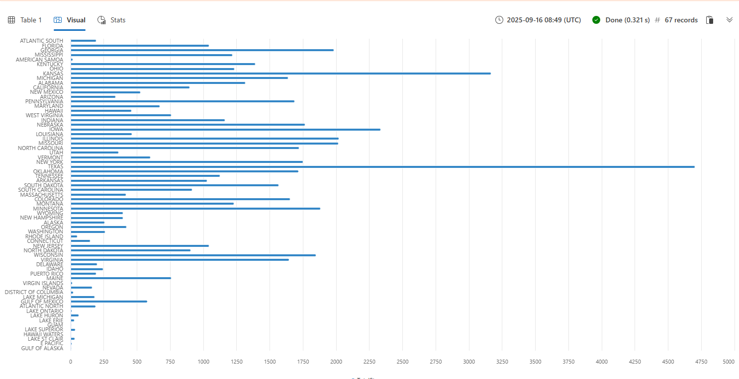
Find the number of events by state using summarize with the count aggregation function.

StormEvents
| summarize TotalStorms = count() by State

Output

State	TotalStorms
TEXAS	4701
KANSAS	3166
IOWA	2337
ILLINOIS	2022
MISSOURI	2016
...	...

Visualize query results

Visualizing query results in a chart or graph can help you identify patterns, trends, and outliers in your data. You can do this with the render operator.

Throughout the tutorial, you'll see examples of how to use render to display your results. For now, let's use render to see the results from the previous query in a bar chart.

StormEvents
| summarize TotalStorms = count() by State
| render barchart

Conditionally count rows

When analyzing your data, use countif() to count rows based on a specific condition to understand how many rows meet the given criteria.

The following query uses countif() to count of storms that caused damage. The query then uses the top operator to filter the results and display the states with the highest amount of crop damage caused by storms.

StormEvents
| summarize StormsWithCropDamage = countif(DamageCrops > 0) by State
| top 5 by StormsWithCropDamage

Output

State	StormsWithCropDamage
IOWA	359
NEBRASKA	201
MISSISSIPPI	105
NORTH CAROLINA	82
MISSOURI	78

Group data into bins

To aggregate by numeric or time values, you'll first want to group the data into bins using the bin() function. Using bin() can help you understand how values are distributed within a certain range and make comparisons between different periods.

The following query counts the number of storms that caused crop damage for each week in 2007. The 7d argument represents a week, as the function requires a valid timespan value.

StormEvents
| where StartTime between (datetime(2007-01-01) .. datetime(2007-12-31)) 
    and DamageCrops > 0
| summarize EventCount = count() by bin(StartTime, 7d)

Output

StartTime	EventCount
2007-01-01T00:00:00Z	16
2007-01-08T00:00:00Z	20
2007-01-29T00:00:00Z	8
2007-02-05T00:00:00Z	1
2007-02-12T00:00:00Z	3
...	...

Add | render timechart to the end of the query to visualize the results.

Calculate the min, max, avg, and sum

To learn more about types of storms that cause crop damage, calculate the min(), max(), and avg() crop damage for each event type, and then sort the result by the average damage.

Note that you can use multiple aggregation functions in a single summarize operator to produce several computed columns.

StormEvents
| where DamageCrops > 0
| summarize
    MaxCropDamage=max(DamageCrops), 
    MinCropDamage=min(DamageCrops), 
    AvgCropDamage=avg(DamageCrops)
    by EventType
| sort by AvgCropDamage

Output

EventType	MaxCropDamage	MinCropDamage	AvgCropDamage
Frost/Freeze	568600000	3000	9106087.5954198465
Wildfire	21000000	10000	7268333.333333333
Drought	700000000	2000	6763977.8761061952
Flood	500000000	1000	4844925.23364486
Thunderstorm Wind	22000000	100	920328.36538461538
...	...	...	...

The results of the previous query indicate that Frost/Freeze events resulted in the most crop damage on average. However, the bin() query showed that events with crop damage mostly took place in the summer months.

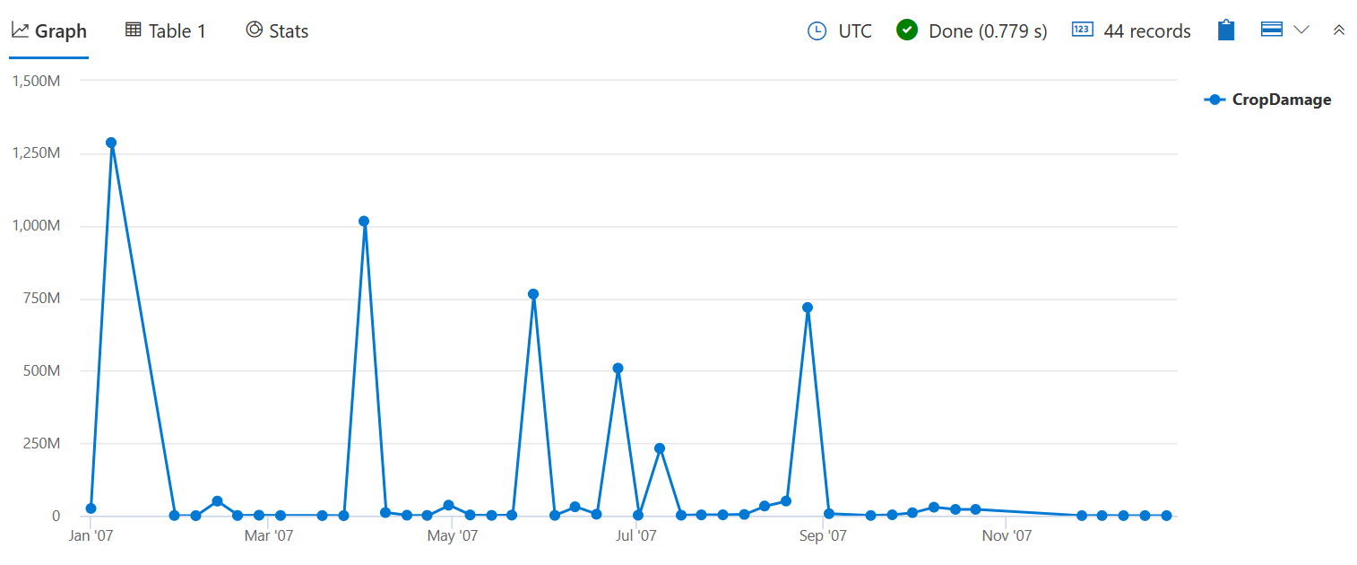
Use sum() to check the total number of damaged crops instead of the amount of events that caused some damage, as done with count() in the previous bin() query.

StormEvents
| where StartTime between (datetime(2007-01-01) .. datetime(2007-12-31)) 
    and DamageCrops > 0
| summarize CropDamage = sum(DamageCrops) by bin(StartTime, 7d)
| render timechart

Now you can see a peak in crop damage in January, which probably was due to Frost/Freeze.

Calculate percentages

Calculating percentages can help you understand the distribution and proportion of different values within your data. This section covers two common methods for calculating percentages with the Kusto Query Language (KQL).

Calculate percentage based on two columns

Use count() and countif to find the percentage of storm events that caused crop damage in each state. First, count the total number of storms in each state. Then, count the number of storms that caused crop damage in each state.

Then, use extend to calculate the percentage between the two columns by dividing the number of storms with crop damage by the total number of storms and multiplying by 100.

To ensure that you get a decimal result, use the todouble() function to convert at least one of the integer count values to a double before performing the division.

StormEvents
| summarize 
    TotalStormsInState = count(),
    StormsWithCropDamage = countif(DamageCrops > 0)
    by State
| extend PercentWithCropDamage = 
    round((todouble(StormsWithCropDamage) / TotalStormsInState * 100), 2)
| sort by StormsWithCropDamage

Output

State	TotalStormsInState	StormsWithCropDamage	PercentWithCropDamage
IOWA	2337	359	15.36
NEBRASKA	1766	201	11.38
MISSISSIPPI	1218	105	8.62
NORTH CAROLINA	1721	82	4.76
MISSOURI	2016	78	3.87
...	...	...	...

Calculate percentage based on table size

To compare the number of storms by event type to the total number of storms in the database, first save the total number of storms in the database as a variable. Let statements are used to define variables within a query.

Since tabular expression statements return tabular results, use the toscalar() function to convert the tabular result of the count() function to a scalar value. Then, the numeric value can be used in the percentage calculation.

let TotalStorms = toscalar(StormEvents | summarize count());
StormEvents
| summarize EventCount = count() by EventType
| project EventType, EventCount, Percentage = todouble(EventCount) / TotalStorms * 100.0

Output

EventType	EventCount	Percentage
Thunderstorm Wind	13015	22.034673077574237
Hail	12711	21.519994582331627
Flash Flood	3688	6.2438627975485055
Drought	3616	6.1219652592015716
Winter Weather	3349	5.669928554498358
...	...	...

Extract unique values

Use make_set() to turn a selection of rows in a table into an array of unique values.

The following query uses make_set() to create an array of the event types that cause deaths in each state. The resulting table is then sorted by the number of storm types in each array.

StormEvents
| where DeathsDirect > 0 or DeathsIndirect > 0
| summarize StormTypesWithDeaths = make_set(EventType) by State
| project State, StormTypesWithDeaths
| sort by array_length(StormTypesWithDeaths)

Output

State	StormTypesWithDeaths
CALIFORNIA	["Thunderstorm Wind","High Surf","Cold/Wind Chill","Strong Wind","Rip Current","Heat","Excessive Heat","Wildfire","Dust Storm","Astronomical Low Tide","Dense Fog","Winter Weather"]
TEXAS	["Flash Flood","Thunderstorm Wind","Tornado","Lightning","Flood","Ice Storm","Winter Weather","Rip Current","Excessive Heat","Dense Fog","Hurricane (Typhoon)","Cold/Wind Chill"]
OKLAHOMA	["Flash Flood","Tornado","Cold/Wind Chill","Winter Storm","Heavy Snow","Excessive Heat","Heat","Ice Storm","Winter Weather","Dense Fog"]
NEW YORK	["Flood","Lightning","Thunderstorm Wind","Flash Flood","Winter Weather","Ice Storm","Extreme Cold/Wind Chill","Winter Storm","Heavy Snow"]
KANSAS	["Thunderstorm Wind","Heavy Rain","Tornado","Flood","Flash Flood","Lightning","Heavy Snow","Winter Weather","Blizzard"]
...	...

Bucket data by condition

The case() function groups data into buckets based on specified conditions. The function returns the corresponding result expression for the first satisfied predicate, or the final else expression if none of the predicates are satisfied.

This example groups states based on the number of storm-related injuries their citizens sustained.

StormEvents
| summarize InjuriesCount = sum(InjuriesDirect) by State
| extend InjuriesBucket = case (
                              InjuriesCount > 50,
                              "Large",
                              InjuriesCount > 10,
                              "Medium",
                              InjuriesCount > 0,
                              "Small",
                              "No injuries"
                          )
| sort by State asc

Output

State	InjuriesCount	InjuriesBucket
ALABAMA	494	Large
ALASKA	0	No injuries
AMERICAN SAMOA	0	No injuries
ARIZONA	6	Small
ARKANSAS	54	Large
ATLANTIC NORTH	15	Medium
...	...	...

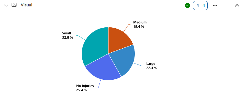
Create a pie chart to visualize the proportion of states that experienced storms resulting in a large, medium, or small number of injuries.

StormEvents
| summarize InjuriesCount = sum(InjuriesDirect) by State
| extend InjuriesBucket = case (
                              InjuriesCount > 50,
                              "Large",
                              InjuriesCount > 10,
                              "Medium",
                              InjuriesCount > 0,
                              "Small",
                              "No injuries"
                          )
| summarize InjuryBucketByState=count() by InjuriesBucket
| render piechart 

Perform aggregations over a sliding window

The following example shows how to summarize columns using a sliding window.

The query calculates the minimum, maximum, and average property damage of tornados, floods, and wildfires using a sliding window of seven days. Each record in the result set aggregates the preceding seven days, and the results contain a record per day in the analysis period.

Here's a step-by-step explanation of the query:

1. Bin each record to a single day relative to windowStart.
2. Add seven days to the bin value to set the end of the range for each record. If the value is out of the range of windowStart and windowEnd, adjust the value accordingly.
3. Create an array of seven days for each record, starting from the current day of the record.
4. Expand the array from step 3 with mv-expand in order to duplicate each record to seven records with one-day intervals between them.
5. Perform the aggregations for each day. Due to step 4, this step actually summarizes the previous seven days.
6. Exclude the first seven days from the final result because there's no seven-day lookback period for them.

let windowStart = datetime(2007-07-01);
let windowEnd = windowStart + 13d;
StormEvents
| where EventType in ("Tornado", "Flood", "Wildfire") 
| extend bin = bin_at(startofday(StartTime), 1d, windowStart) // 1
| extend endRange = iff(bin + 7d > windowEnd, windowEnd, 
                      iff(bin + 7d - 1d < windowStart, windowStart, 
                        iff(bin + 7d - 1d < bin, bin, bin + 7d - 1d))) // 2
| extend range = range(bin, endRange, 1d) // 3
| mv-expand range to typeof(datetime) // 4
| summarize min(DamageProperty), max(DamageProperty), round(avg(DamageProperty)) by Timestamp=bin_at(range, 1d, windowStart), EventType // 5
| where Timestamp >= windowStart + 7d; // 6

Output

The following result table is truncated. To see the full output, run the query.

Timestamp	EventType	min_DamageProperty	max_DamageProperty	avg_DamageProperty
2007-07-08T00:00:00Z	Tornado	0	30000	6905
2007-07-08T00:00:00Z	Flood	0	200000	9261
2007-07-08T00:00:00Z	Wildfire	0	200000	14033
2007-07-09T00:00:00Z	Tornado	0	100000	14783
2007-07-09T00:00:00Z	Flood	0	200000	12529
2007-07-09T00:00:00Z	Wildfire	0	200000	14033
2007-07-10T00:00:00Z	Tornado	0	100000	31400
2007-07-10T00:00:00Z	Flood	0	200000	12263
2007-07-10T00:00:00Z	Wildfire	0	200000	11694
...	...	...

Next step

Now that you're familiar with common query operators and aggregation functions, go on to the next tutorial to learn how to join data from multiple tables.