应用从自变量 (x_series) 到因变量 (y_series) 的多项式回归。 此函数获取包含多个序列(动态数值阵列)的表,并使用多项式回归为每个序列生成拟合效果最佳的高阶多项式。
提示
- 对于间距均匀的序列(由 make-series 运算符创建)的线性回归,请使用更简单的函数 series_fit_line()。 请参阅示例 2。
- 如果提供了 x_series,并且回归程度很高,请考虑规范化为 [0-1] 范围。 请参阅示例 3。
- 如果 x_series 的类型为 datetime,则必须将其转换为 double 类型,并对其进行规范化。 请参阅示例 3。
- 有关使用内联 Python 实现多项式回归的参考,请参阅 series_fit_poly_fl()。
语法
T | extend series_fit_poly(y_series [, x_series, degree ])
详细了解语法约定。
参数
| 客户 | 类型 | 必需 | 说明 |
|---|---|---|---|
| y_series | dynamic |
✔️ | 包含因变量的数值数组。 |
| x_series | dynamic |
包含自变量的数值数组。 仅对于间距不均匀的序列是必需的。 如果未指定,则将其设置为默认值 [1, 2, ..., length(y_series)]。 | |
| degree | 要拟合的多项式所需的阶。 例如,1 用于线性回归,2 用于二次回归,等等。 默认为 1,表示线性回归。 |
返回
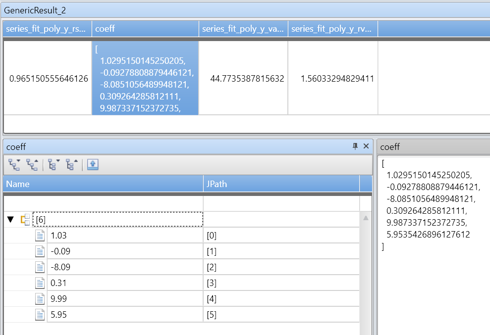
series_fit_poly() 函数返回以下列:
rsquare:r-square 是用于衡量拟合质量的标准。 此值是 [0-1] 范围内的数字,其中 1 表示拟合度最好,0 表示数据无序,与任何直线均不拟合。coefficients:数值阵列,保存给定拟合度的最佳拟合多项式的系数,从最高幂系数到最低幂系数进行排序。variance:因变量 (y_series) 的方差。rvariance:剩余方差,即输入数据值和近似数据值之间的方差。poly_fit:数值阵列,其中包含拟合度最好的多项式的一系列值。 序列长度等于因变量 (y_series) 的长度。 该值用于绘制图表。
示例
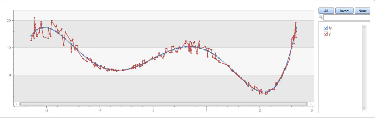
示例 1
x 轴和 y 轴上有干扰信息的第 5 阶多项式:
range x from 1 to 200 step 1
| project x = rand()*5 - 2.3
| extend y = pow(x, 5)-8*pow(x, 3)+10*x+6
| extend y = y + (rand() - 0.5)*0.5*y
| summarize x=make_list(x), y=make_list(y)
| extend series_fit_poly(y, x, 5)
| project-rename fy=series_fit_poly_y_poly_fit, coeff=series_fit_poly_y_coefficients
|fork (project x, y, fy) (project-away x, y, fy)
| render linechart
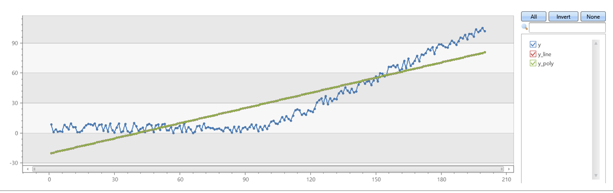
示例 2
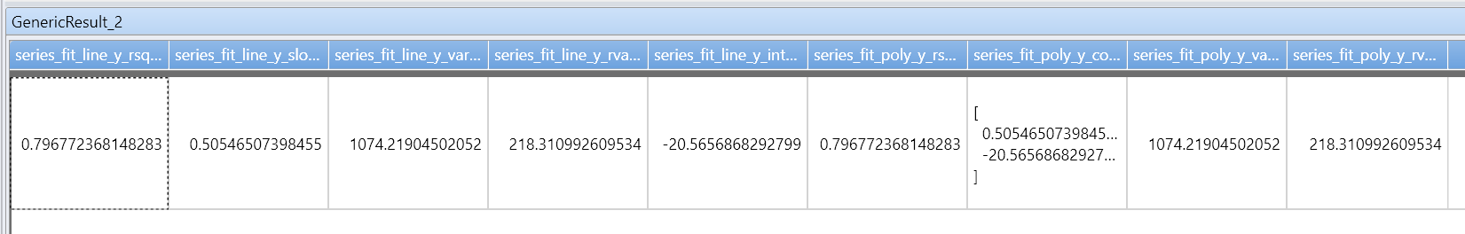
验证拟合度 = 1 的 series_fit_poly 是否与 series_fit_line 匹配:
demo_series1
| extend series_fit_line(y)
| extend series_fit_poly(y)
| project-rename y_line = series_fit_line_y_line_fit, y_poly = series_fit_poly_y_poly_fit
| fork (project x, y, y_line, y_poly) (project-away id, x, y, y_line, y_poly)
| render linechart with(xcolumn=x, ycolumns=y, y_line, y_poly)
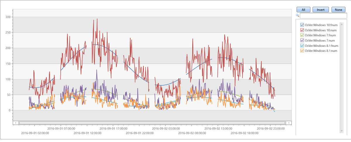
示例 3
不规律(间距不均匀)的时序:
//
//  x-axis must be normalized to the range [0-1] if either degree is relatively big (>= 5) or original x range is big.
//  so if x is a time axis it must be normalized as conversion of timestamp to long generate huge numbers (number of 100 nano-sec ticks from 1/1/1970)
//
//  Normalization: x_norm = (x - min(x))/(max(x) - min(x))
//
irregular_ts
| extend series_stats(series_add(TimeStamp, 0))                                                                 //  extract min/max of time axis as doubles
| extend x = series_divide(series_subtract(TimeStamp, series_stats__min), series_stats__max-series_stats__min)  // normalize time axis to [0-1] range
| extend series_fit_poly(num, x, 8)
| project-rename fnum=series_fit_poly_num_poly_fit
| render timechart with(ycolumns=num, fnum)