Nota:
El acceso a esta página requiere autorización. Puede intentar iniciar sesión o cambiar directorios.
El acceso a esta página requiere autorización. Puede intentar cambiar los directorios.
本文介绍如何使用 Apache Spark MLlib 创建在 Azure 开放数据集上进行简单预测分析的机器学习应用程序。 Spark 提供内置的机器学习库。 此示例通过逻辑回归使用 分类 。
SparkML 和 MLlib 是核心 Spark 库,提供许多可用于机器学习任务的实用工具,包括适用于以下任务的实用工具:
- 分类
- 回归
- 集群
- 主题建模
- 单一值分解(SVD)和主体组件分析(PCA)
- 假设测试和计算示例统计信息
了解分类和逻辑回归
分类是一项常用的机器学习任务,是将输入数据排序到类别的过程。 分类算法的工作是了解如何将 标签 分配给你提供的输入数据。 例如,可以将接受股票信息的机器学习算法视为输入,并将股票划分为两类:应出售的股票和应保留的股票。
逻辑回归 是一种可用于分类的算法。 Spark 的逻辑回归 API 可用于 二元分类,或将输入数据分类为两个组之一。 有关逻辑回归的详细信息,请参阅 Wikipedia。
总之,逻辑回归过程生成一个 逻辑函数 ,可用于预测输入向量属于一组或其他组的概率。
纽约出租车数据的预测分析示例
在此示例中,使用 Spark 对来自纽约的出租车行程小费数据执行一些预测分析。 数据通过 Azure 开放数据集提供。 数据集的此子集包含有关黄色出租车行程的信息,包括有关每个行程、开始时间和结束时间和位置、成本和其他有趣属性的信息。
重要
从存储位置拉取这些数据可能会产生额外的费用。
在以下步骤中,你将开发一个模型来预测某个行程是否包含小费。
创建 Apache Spark 机器学习模型
使用 PySpark 内核创建笔记本。 有关说明,请参阅创建笔记本。
导入此应用程序所需的类型。 将以下代码复制并粘贴到空单元格中,然后按 Shift+Enter。 或者使用代码左侧的蓝色播放图标运行该单元格。
import matplotlib.pyplot as plt
from datetime import datetime
from dateutil import parser
from pyspark.sql.functions import unix_timestamp, date_format, col, when
from pyspark.ml import Pipeline
from pyspark.ml import PipelineModel
from pyspark.ml.feature import RFormula
from pyspark.ml.feature import OneHotEncoder, StringIndexer, VectorIndexer
from pyspark.ml.classification import LogisticRegression
from pyspark.mllib.evaluation import BinaryClassificationMetrics
from pyspark.ml.evaluation import BinaryClassificationEvaluator
由于使用的是 PySpark 内核,因此不需要显式创建任何上下文。 运行第一个代码单元格时,系统会自动创建 Spark 上下文。
构造输入数据帧
由于原始数据采用 Parquet 格式,因此可以使用 Spark 上下文将文件作为数据帧直接拉取到内存中。 尽管以下步骤中的代码使用默认选项,但如果需要,可以强制映射数据类型和其他架构属性。
运行以下行,通过将代码粘贴到新单元格来创建 Spark 数据帧。 此步骤通过开放数据集 API 检索数据。 提取所有这些数据会生成大约 15 亿行。
根据无服务器 Apache Spark 池的大小,原始数据可能过大或处理所需时间过长。 可以将此数据筛选为更小的数据集。 下面的代码示例使用
start_date并end_date应用返回单个月数据的筛选器。from azureml.opendatasets import NycTlcYellow from datetime import datetime from dateutil import parser end_date = parser.parse('2018-05-08 00:00:00') start_date = parser.parse('2018-05-01 00:00:00') nyc_tlc = NycTlcYellow(start_date=start_date, end_date=end_date) filtered_df = spark.createDataFrame(nyc_tlc.to_pandas_dataframe())简单筛选的缺点是,从统计的角度来看,它可能会对数据产生偏见。 另一种方法是使用 Spark 中内置的采样。
以下代码将数据集减少到大约 2,000 行(如果应用在上述代码之后)。 可以使用此采样步骤而不是简单筛选器,也可以与简单筛选器结合使用。
# To make development easier, faster, and less expensive, downsample for now
sampled_taxi_df = filtered_df.sample(True, 0.001, seed=1234)
现在可以查看数据以查看读取的内容。 通常,最好根据数据集的大小来查看具有子集而不是完整集的数据。
以下代码提供了两种方法来查看数据。 第一种方法是基本的。 第二种方法提供更丰富的网格体验,以及以图形方式可视化数据的功能。
#sampled_taxi_df.show(5)
display(sampled_taxi_df)
可能需要在本地工作区中缓存数据集,具体取决于生成的数据集的大小,并且需要多次试验或运行笔记本。 有三种方法可以执行显式缓存:
- 将 DataFrame 本地保存为文件。
- 将 DataFrame 保存为临时表或视图。
- 将 DataFrame 保存为永久表。
以下代码示例中包括这两种方法的前两种方法。
创建临时表或视图可提供对数据的不同访问路径,但它仅持续到 Spark 实例会话的持续时间。
sampled_taxi_df.createOrReplaceTempView("nytaxi")
准备数据
其原始形式的数据通常不适合直接传递到模型。 必须对数据执行一系列操作,才能使其达到模型能够使用的状态。
在以下代码中,你将执行四类作:
- 通过筛选删除离群值或错误值。
- 删除不需要的列。
- 创建从原始数据派生的新列,使模型更高效地工作。 此操作有时称为特征化。
- 标记。 由于要进行二元分类(给定行程中会有小费或不进行),因此需要将小费金额转换为 0 或 1 值。
taxi_df = sampled_taxi_df.select('totalAmount', 'fareAmount', 'tipAmount', 'paymentType', 'rateCodeId', 'passengerCount'\
                                , 'tripDistance', 'tpepPickupDateTime', 'tpepDropoffDateTime'\
                                , date_format('tpepPickupDateTime', 'hh').alias('pickupHour')\
                                , date_format('tpepPickupDateTime', 'EEEE').alias('weekdayString')\
                                , (unix_timestamp(col('tpepDropoffDateTime')) - unix_timestamp(col('tpepPickupDateTime'))).alias('tripTimeSecs')\
                                , (when(col('tipAmount') > 0, 1).otherwise(0)).alias('tipped')
                                )\
                        .filter((sampled_taxi_df.passengerCount > 0) & (sampled_taxi_df.passengerCount < 8)\
                                & (sampled_taxi_df.tipAmount >= 0) & (sampled_taxi_df.tipAmount <= 25)\
                                & (sampled_taxi_df.fareAmount >= 1) & (sampled_taxi_df.fareAmount <= 250)\
                                & (sampled_taxi_df.tipAmount < sampled_taxi_df.fareAmount)\
                                & (sampled_taxi_df.tripDistance > 0) & (sampled_taxi_df.tripDistance <= 100)\
                                & (sampled_taxi_df.rateCodeId <= 5)
                                & (sampled_taxi_df.paymentType.isin({"1", "2"}))
                                )
然后,对数据进行第二次传递,以添加最终功能。
taxi_featurised_df = taxi_df.select('totalAmount', 'fareAmount', 'tipAmount', 'paymentType', 'passengerCount'\
                                                , 'tripDistance', 'weekdayString', 'pickupHour','tripTimeSecs','tipped'\
                                                , when((taxi_df.pickupHour <= 6) | (taxi_df.pickupHour >= 20),"Night")\
                                                .when((taxi_df.pickupHour >= 7) & (taxi_df.pickupHour <= 10), "AMRush")\
                                                .when((taxi_df.pickupHour >= 11) & (taxi_df.pickupHour <= 15), "Afternoon")\
                                                .when((taxi_df.pickupHour >= 16) & (taxi_df.pickupHour <= 19), "PMRush")\
                                                .otherwise(0).alias('trafficTimeBins')
                                              )\
                                       .filter((taxi_df.tripTimeSecs >= 30) & (taxi_df.tripTimeSecs <= 7200))
创建逻辑回归模型
最后一项任务是将标记的数据转换为可通过逻辑回归分析的格式。 逻辑回归算法的输入必须是一组 标签/特征向量对,其中 特征向量 是表示输入点的数字向量。
因此,需要将分类列转换为数字。 具体而言,需要将 trafficTimeBins 列和 weekdayString 列转换为整数表示形式。 有多种方法可以执行转换。 以下示例采用 OneHotEncoder 常见方法。
# Because the sample uses an algorithm that works only with numeric features, convert them so they can be consumed
sI1 = StringIndexer(inputCol="trafficTimeBins", outputCol="trafficTimeBinsIndex")
en1 = OneHotEncoder(dropLast=False, inputCol="trafficTimeBinsIndex", outputCol="trafficTimeBinsVec")
sI2 = StringIndexer(inputCol="weekdayString", outputCol="weekdayIndex")
en2 = OneHotEncoder(dropLast=False, inputCol="weekdayIndex", outputCol="weekdayVec")

# Create a new DataFrame that has had the encodings applied
encoded_final_df = Pipeline(stages=[sI1, en1, sI2, en2]).fit(taxi_featurised_df).transform(taxi_featurised_df)
此操作将生成一个新的 DataFrame,其中所有列都采用正确格式,以便用于训练模型。
训练逻辑回归模型
第一个任务是将数据集拆分为训练集和测试或验证集。 此处的拆分是任意的。 试验不同的拆分设置,以查看它们是否影响模型。
# Decide on the split between training and testing data from the DataFrame
trainingFraction = 0.7
testingFraction = (1-trainingFraction)
seed = 1234

# Split the DataFrame into test and training DataFrames
train_data_df, test_data_df = encoded_final_df.randomSplit([trainingFraction, testingFraction], seed=seed)
现在有两个 DataFrame,下一个任务是创建模型公式,并针对训练数据帧运行它。 然后,可以针对测试数据帧进行验证。 试验不同版本的模型公式以查看不同组合的影响。
注释
若要保存模型,请将 存储 Blob 数据参与者 角色分配给 Azure SQL 数据库服务器资源范围。 有关详细步骤,请参阅使用 Azure 门户分配 Azure 角色。 只有拥有所有者权限的成员才能执行此步骤。
## Create a new logistic regression object for the model
logReg = LogisticRegression(maxIter=10, regParam=0.3, labelCol = 'tipped')

## The formula for the model
classFormula = RFormula(formula="tipped ~ pickupHour + weekdayVec + passengerCount + tripTimeSecs + tripDistance + fareAmount + paymentType+ trafficTimeBinsVec")

## Undertake training and create a logistic regression model
lrModel = Pipeline(stages=[classFormula, logReg]).fit(train_data_df)

## Saving the model is optional, but it's another form of inter-session cache
datestamp = datetime.now().strftime('%m-%d-%Y-%s')
fileName = "lrModel_" + datestamp
logRegDirfilename = fileName
lrModel.save(logRegDirfilename)

## Predict tip 1/0 (yes/no) on the test dataset; evaluation using area under ROC
predictions = lrModel.transform(test_data_df)
predictionAndLabels = predictions.select("label","prediction").rdd
metrics = BinaryClassificationMetrics(predictionAndLabels)
print("Area under ROC = %s" % metrics.areaUnderROC)
此单元格的输出为:
Area under ROC = 0.9779470729751403
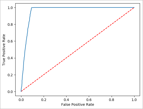
创建预测的可视表示形式
现在可以构造最终的可视化效果,以帮助你推理此测试结果。 ROC 曲线是查看结果的一种方法。
## Plot the ROC curve; no need for pandas, because this uses the modelSummary object
modelSummary = lrModel.stages[-1].summary

plt.plot([0, 1], [0, 1], 'r--')
plt.plot(modelSummary.roc.select('FPR').collect(),
         modelSummary.roc.select('TPR').collect())
plt.xlabel('False Positive Rate')
plt.ylabel('True Positive Rate')
plt.show()
关闭 Spark 实例
运行完应用程序后,关闭笔记本以关闭选项卡释放资源。或者从笔记本底部的状态面板中选择 “结束会话 ”。
另请参阅
后续步骤
注释
某些官方 Apache Spark 文档依赖于使用 Spark 控制台,该控制台在 Azure Synapse Analytics 中的 Apache Spark 上不可用。 请改用笔记本体验。