云服务和 IoT 设备生成用于监视服务运行状况、业务流程和使用情况趋势的遥测数据。 时序分析有助于发现每个指标的基线模式的偏差。
Kusto 查询语言(KQL)包括对创建、操作和分析多个时序的原生支持。 使用 KQL 创建和分析数千个时序(以秒为单位)进行近实时监视。
本文介绍 KQL 时序异常情况检测和预测功能。 这些函数使用可靠的已知分解模型,将每个时序拆分为季节性、趋势和残差组件。 通过在残差组件中查找离群值来检测异常。 通过推断季节性和趋势组件来预测。 KQL 添加了自动季节性检测、可靠的离群值分析和矢量化实现,以秒为单位处理数千个时序。
先决条件
- 使用Microsoft帐户或 Microsoft Entra 用户标识。 不需要 Azure 订阅。
- 阅读有关时序分析中的时间序列功能。
时序分解模型
用于时序预测和异常情况检测的 KQL 本机实现使用已知的分解模型。 将此模型用于具有周期性行为和趋势行为的时序(例如服务流量、组件检测信号和定期 IoT 度量)来预测将来的值并检测异常。 回归假定余数在移除季节性和趋势组件后是随机的。 预测季节性和趋势组件(基线)的未来值,并忽略残差。 通过对残差组件进行离群值分析来检测异常。
使用该 series_decompose() 函数创建分解模型。 它将每个时序分解为季节性、趋势、残差和基线组件。
示例:分解内部 Web 服务流量:
let min_t = datetime(2017-01-05);
let max_t = datetime(2017-02-03 22:00);
let dt = 2h;
demo_make_series2
| make-series num=avg(num) on TimeStamp from min_t to max_t step dt by sid
| where sid == 'TS1'   // Select a single time series for cleaner visualization
| extend (baseline, seasonal, trend, residual) = series_decompose(num, -1, 'linefit')  // Decompose each time series into seasonal, trend, residual, and baseline (seasonal + trend)
| render timechart with(title='Web app traffic for one month, decomposition', ysplit=panels)
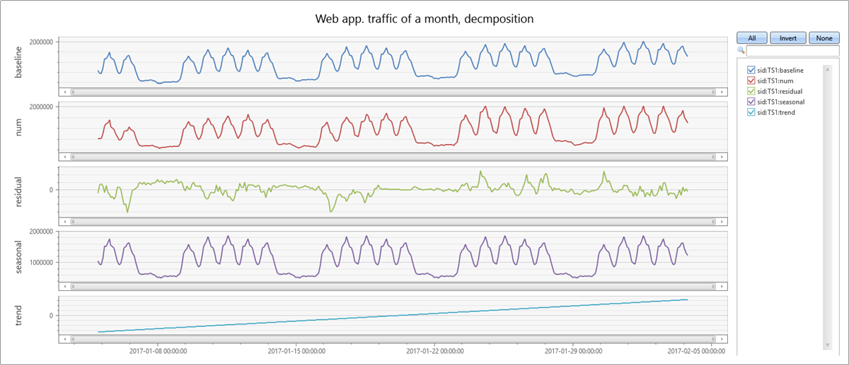
- 原始时序带有 num(如红色所示)标签。
- 该过程使用
series_periods_detect()函数自动检测季节性,并提取 季节性 模式(紫色)。 - 从原始时序中减去季节性模式,然后使用函数运行线性回归
series_fit_line()以查找 趋势 分量(浅蓝色)。 - 该函数减去趋势,其余部分为 残差 部分(绿色)。
- 最后,添加季节性和趋势组件以生成 基线 (蓝色)。
时序异常情况检测
函数 series_decompose_anomalies() 查找一组时序中的异常点。 此函数调用 series_decompose() 来生成分解模型,然后对残余组件运行 series_outliers()。
series_outliers() 使用 Tukey 隔离测试计算残余组件的每个点的异常评分。 异常评分大于 1.5 或小于 -1.5 分别表示异常有轻微的上升或下降。 异常评分大于 3.0 或小于 -3.0 表示明显的异常。
使用以下查询可以检测内部 Web 服务流量的异常:
let min_t = datetime(2017-01-05);
let max_t = datetime(2017-02-03 22:00);
let dt = 2h;
demo_make_series2
| make-series num=avg(num) on TimeStamp from min_t to max_t step dt by sid
| where sid == 'TS1'   //  select a single time series for a cleaner visualization
| extend (anomalies, score, baseline) = series_decompose_anomalies(num, 1.5, -1, 'linefit')
| render anomalychart with(anomalycolumns=anomalies, title='Web app. traffic of a month, anomalies') //use "| render anomalychart with anomalycolumns=anomalies" to render the anomalies as bold points on the series charts.
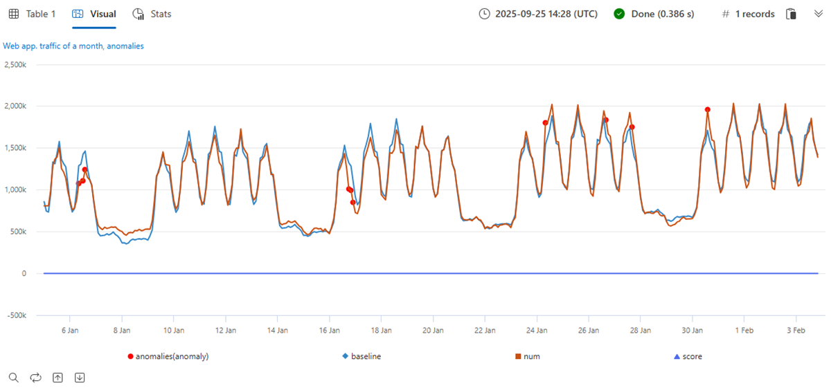
- 原始时序(如红色所示)。
- 基线(季节性 + 趋势)组件(如蓝色所示)。
- 原始时序顶层的异常点(如紫色所示)。 异常点明显偏离于预期的基线值。
时序预测
函数 series_decompose_forecast() 预测一组时序的未来值。 此函数调用 series_decompose() 生成分解模型,然后针对每个时序,推断未来的基线组件。
使用以下查询可以预测下一周的 Web 服务流量:
let min_t = datetime(2017-01-05);
let max_t = datetime(2017-02-03 22:00);
let dt = 2h;
let horizon=7d;
demo_make_series2
| make-series num=avg(num) on TimeStamp from min_t to max_t+horizon step dt by sid
| where sid == 'TS1'   //  select a single time series for a cleaner visualization
| extend forecast = series_decompose_forecast(num, toint(horizon/dt))
| render timechart with(title='Web app. traffic of a month, forecasting the next week by Time Series Decomposition')
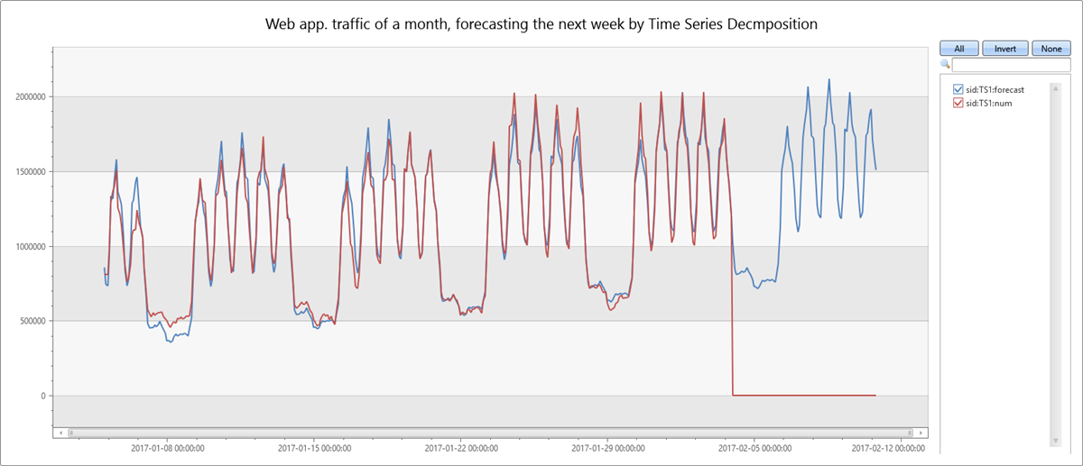
- 原始指标(如红色所示)。 未来值缺失,已按默认设置为 0。
- 推断基线组件(蓝色)以预测下一周的值。
可伸缩性
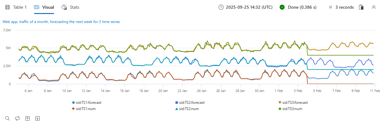
Kusto 查询语言语法支持通过单个调用来处理多个时序。 其独特的优化实现可以提高性能,在近实时方案中监视数千个计数器时,若要有效进行异常情况检测和预测,这种优势非常关键。
以下查询显示同时处理三个时序的结果:
let min_t = datetime(2017-01-05);
let max_t = datetime(2017-02-03 22:00);
let dt = 2h;
let horizon=7d;
demo_make_series2
| make-series num=avg(num) on TimeStamp from min_t to max_t+horizon step dt by sid
| extend offset=case(sid=='TS3', 4000000, sid=='TS2', 2000000, 0)   //  add artificial offset for easy visualization of multiple time series
| extend num=series_add(num, offset)
| extend forecast = series_decompose_forecast(num, toint(horizon/dt))
| render timechart with(title='Web app. traffic of a month, forecasting the next week for 3 time series')
摘要
本文档详细介绍了用于时序异常情况检测和预测的本机 KQL 函数。 每个原始时序都分解为季节性、趋势和残差组件,用于检测异常和/或预测。 这些功能可用于近实时监视方案,例如故障检测、预测性维护以及需求和负载预测。
相关内容
- 了解 KQL 的异常诊断功能