Note
Access to this page requires authorization. You can try signing in or changing directories.
Access to this page requires authorization. You can try changing directories.
Switch services using the Version drop-down list. Learn more about navigation.
Applies to: ✅ Azure Data Explorer ✅ Azure Monitor ✅ Microsoft Sentinel
Applies a polynomial regression from an independent variable (x_series) to a dependent variable (y_series). This function takes a table containing multiple series (dynamic numerical arrays) and generates the best fit high-order polynomial for each series using polynomial regression.
Tip
- For linear regression of an evenly spaced series, as created by make-series operator, use the simpler function series_fit_line(). See Example 2.
- If x_series is supplied, and the regression is done for a high degree, consider normalizing to the [0-1] range. See Example 3.
- If x_series is of datetime type, it must be converted to double and normalized. See Example 3.
- For reference implementation of polynomial regression using inline Python, see series_fit_poly_fl().
Syntax
T | extend series_fit_poly(y_series [, x_series, degree ])
Learn more about syntax conventions.
Parameters
| Name | Type | Required | Description |
|---|---|---|---|
| y_series | dynamic |
✔️ | An array of numeric values containing the dependent variable. |
| x_series | dynamic |
An array of numeric values containing the independent variable. Required only for unevenly spaced series. If not specified, it's set to a default value of [1, 2, ..., length(y_series)]. | |
| degree | The required order of the polynomial to fit. For example, 1 for linear regression, 2 for quadratic regression, and so on. Defaults to 1, which indicates linear regression. |
Returns
The series_fit_poly() function returns the following columns:
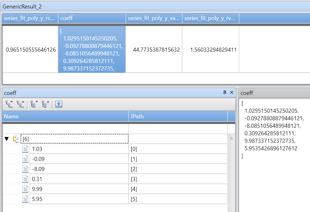
rsquare: r-square is a standard measure of the fit quality. The value's a number in the range [0-1], where 1 - is the best possible fit, and 0 means the data is unordered and doesn't fit any line.coefficients: Numerical array holding the coefficients of the best fitted polynomial with the given degree, ordered from the highest power coefficient to the lowest.variance: Variance of the dependent variable (y_series).rvariance: Residual variance that is the variance between the input data values the approximated ones.poly_fit: Numerical array holding a series of values of the best fitted polynomial. The series length is equal to the length of the dependent variable (y_series). The value's used for charting.
Examples
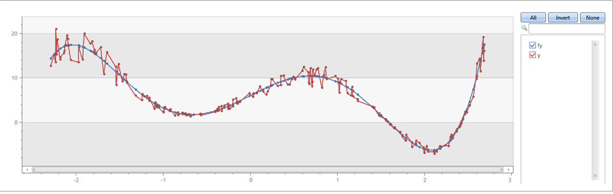
Example 1
A fifth order polynomial with noise on x & y axes:
range x from 1 to 200 step 1
| project x = rand()*5 - 2.3
| extend y = pow(x, 5)-8*pow(x, 3)+10*x+6
| extend y = y + (rand() - 0.5)*0.5*y
| summarize x=make_list(x), y=make_list(y)
| extend series_fit_poly(y, x, 5)
| project-rename fy=series_fit_poly_y_poly_fit, coeff=series_fit_poly_y_coefficients
|fork (project x, y, fy) (project-away x, y, fy)
| render linechart
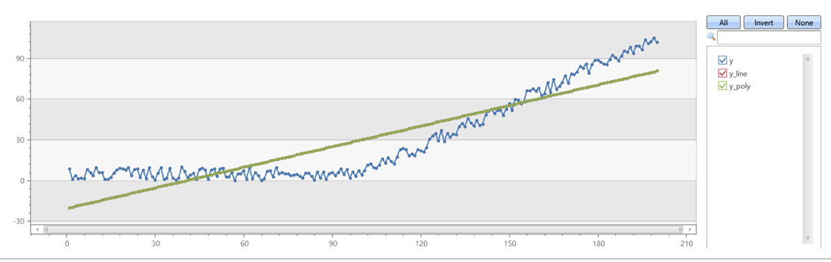
Example 2
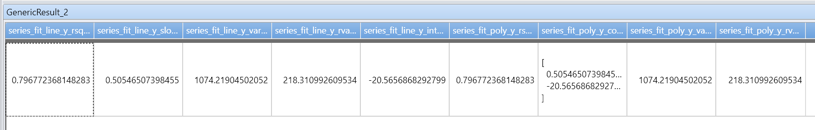
Verify that series_fit_poly with degree=1 matches series_fit_line:
demo_series1
| extend series_fit_line(y)
| extend series_fit_poly(y)
| project-rename y_line = series_fit_line_y_line_fit, y_poly = series_fit_poly_y_poly_fit
| fork (project x, y, y_line, y_poly) (project-away id, x, y, y_line, y_poly)
| render linechart with(xcolumn=x, ycolumns=y, y_line, y_poly)
Example 3
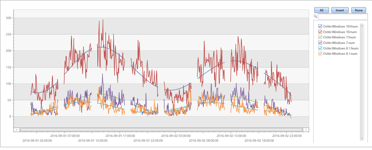
Irregular (unevenly spaced) time series:
//
//  x-axis must be normalized to the range [0-1] if either degree is relatively big (>= 5) or original x range is big.
//  so if x is a time axis it must be normalized as conversion of timestamp to long generate huge numbers (number of 100 nano-sec ticks from 1/1/1970)
//
//  Normalization: x_norm = (x - min(x))/(max(x) - min(x))
//
irregular_ts
| extend series_stats(series_add(TimeStamp, 0))                                                                 //  extract min/max of time axis as doubles
| extend x = series_divide(series_subtract(TimeStamp, series_stats__min), series_stats__max-series_stats__min)  // normalize time axis to [0-1] range
| extend series_fit_poly(num, x, 8)
| project-rename fnum=series_fit_poly_num_poly_fit
| render timechart with(ycolumns=num, fnum)