教程：创建地理空间可视化效果

本教程面向想要利用 Kusto 查询语言 (KQL) 进行地理空间可视化的用户。 地理空间聚类是基于地理位置组织和分析数据的一种方式。 KQL 提供多种用于执行地理空间聚类分析的方法，以及用于创建地理空间可视化效果的工具。

本教程介绍以下操作：

在地图上绘制点

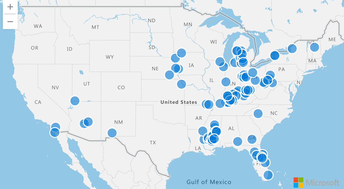
若要将地图上的点可视化，请使用 project 选择包含经度的列，并选择包含纬度的列。 然后，使用 render 在 kind 设置为 map 的散点图中查看结果。

StormEvents
| take 100
| project BeginLon, BeginLat
| render scatterchart with (kind = map)

绘制多个点系列

若要将多个点系列可视化，请使用 project 选择经度和纬度，以及用于定义系列的第三列。

在以下查询中，系列为 EventType。 这些点根据其 EventType 采用不同的配色。选择这些点后，将显示 EventType 列的内容。

StormEvents
| take 100
| project BeginLon, BeginLat, EventType
| render scatterchart with (kind = map)

还可以在执行 render 时显式指定 xcolumn（经度）、ycolumn（纬度）和 series。 如果结果中的列数超过经度、纬度和系列列数，必须指定这些值。

StormEvents
| take 100
| render scatterchart with (kind = map, xcolumn = BeginLon, ycolumns = BeginLat, series = EventType)

使用 GeoJSON 值在地图上绘制点

动态 GeoJSON 值可以更改或更新，通常用于实时地图应用程序。 使用动态 GeoJSON 值在地图上绘制点可以获得更高的灵活性，并可以更好地控制地图上数据的表示，而使用普通的纬度和经度值做不到这一点。

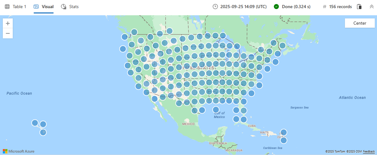
以下查询使用 geo_point_to_s2cell 和 geo_s2cell_to_central_point 在散点图中绘制风暴事件。

StormEvents
| project BeginLon, BeginLat
| summarize by hash=geo_point_to_s2cell(BeginLon, BeginLat, 5)
| project point = geo_s2cell_to_central_point(hash)
| project lng = toreal(point.coordinates[0]), lat = toreal(point.coordinates[1])
| render scatterchart with (kind = map)

使用大小可变的气泡表示数据点

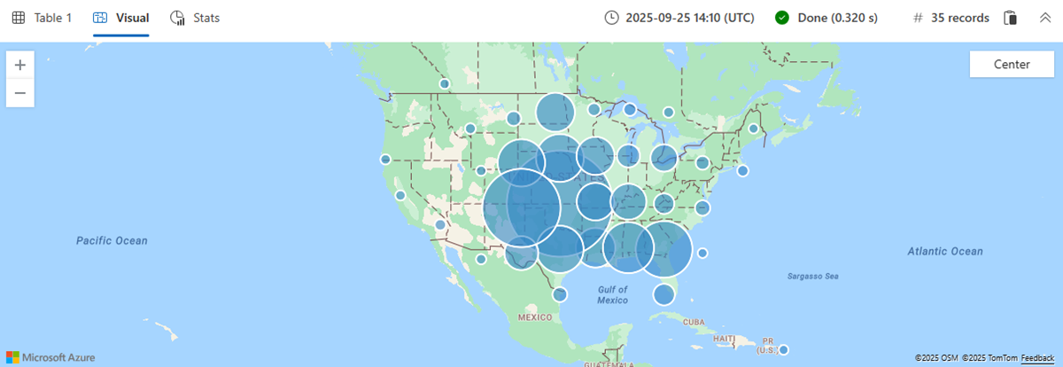
通过在每个聚类中执行聚合然后绘制聚类的中心点，来可视化数据点的分布。

例如，以下查询筛选“龙卷风”(Tornado) 事件类型的所有风暴事件。 然后它根据事件的经度和纬度将事件分组为聚类，统计每个聚类中的事件数，投影聚类的中心点，然后呈现地图以可视化结果。 根据较大的气泡，可以清楚地看到龙卷风发生次数最多的区域。

StormEvents
| where EventType == "Tornado"
| project BeginLon, BeginLat
| where isnotnull(BeginLat) and isnotnull(BeginLon)
| summarize count_summary=count() by hash = geo_point_to_s2cell(BeginLon, BeginLat, 4)
| project geo_s2cell_to_central_point(hash), count_summary
| extend Events = "count"
| render piechart with (kind = map)

显示特定区域中的点

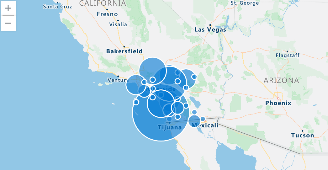
使用多边形定义区域，并使用 geo_point_in_polygon 函数筛选该区域中发生的事件。

以下查询定义一个表示南加州区域的多边形，并筛选该区域中的风暴事件。 然后它将事件分组为聚类，统计每个聚类中的事件数，投影聚类的中心点，然后呈现地图以可视化聚类。

let southern_california = dynamic({
    "type": "Polygon",
    "coordinates": [[[-119.5, 34.5], [-115.5, 34.5], [-115.5, 32.5], [-119.5, 32.5], [-119.5, 34.5]]
    ]});
StormEvents
| where geo_point_in_polygon(BeginLon, BeginLat, southern_california)
| project BeginLon, BeginLat
| summarize count_summary = count() by hash = geo_point_to_s2cell(BeginLon, BeginLat, 8)
| project geo_s2cell_to_central_point(hash), count_summary
| extend Events = "count"
| render piechart with (kind = map)

显示 LineString 上的附近点

以下查询查找沿指定的 LineString（表示已定义路径）发生的附近暴风雨事件。 在本例中，LineString 是通往 Key West 的道路。 geo_distance_point_to_line() 函数用于根据暴风雨事件与所定义 LineString 的邻近性来筛选这些事件。 如果事件位于 LineString 的 500 米范围内，则会在地图上呈现该事件。

let roadToKeyWest = dynamic({
"type":"linestring",
"coordinates":[
          [
            -81.79595947265625,
            24.56461038017685
          ],
          [
            -81.595458984375,
            24.627044746156027
          ],
          [
            -81.52130126953125,
            24.666986385216273
          ],
          [
            -81.35650634765625,
            24.66449040712424
          ],
          [
            -81.32354736328125,
            24.647017162630366
          ],
          [
            -80.8099365234375,
            24.821639356846607
          ],
          [
            -80.62042236328125,
            24.93127614538456
          ],
          [
            -80.37872314453125,
            25.175116531621764
          ],
          [
            -80.42266845703124,
            25.19251511519153
          ],
          [
            -80.4803466796875,
            25.46063471847754
          ]
        ]});
StormEvents
| where isnotempty(BeginLat) and isnotempty(BeginLon)
| project BeginLon, BeginLat, EventType
| where geo_distance_point_to_line(BeginLon, BeginLat, roadToKeyWest) < 500
| render scatterchart with (kind=map)

显示多边形内的附近点

以下查询查找指定多边形内发生的附近暴风雨事件。 在本例中，多边形是通往 Key West 的道路。 geo_distance_point_to_polygon() 函数用于根据暴风雨事件与所定义多边形的邻近性来筛选这些事件。 如果事件位于多边形的 500 米范围内，则会在地图上呈现该事件。

let roadToKeyWest = dynamic({
"type":"polygon",
"coordinates":[
          [
            [
              -80.08209228515625,
              25.39117928167583
            ],
            [
              -80.4913330078125,
              25.517657429994035
            ],
            [
              -80.57922363281249,
              25.477992320574817
            ],
            [
              -82.188720703125,
              24.632038149596895
            ],
            [
              -82.1942138671875,
              24.53712939907993
            ],
            [
              -82.13104248046875,
              24.412140070651528
            ],
            [
              -81.81243896484375,
              24.43714786161562
            ],
            [
              -80.58746337890625,
              24.794214972389486
            ],
            [
              -80.08209228515625,
              25.39117928167583
            ]
          ]
        ]});
StormEvents
| where isnotempty(BeginLat) and isnotempty(BeginLon)
| project BeginLon, BeginLat, EventType
| where geo_distance_point_to_polygon(BeginLon, BeginLat, roadToKeyWest) < 500
| render scatterchart with (kind=map)

根据地理空间数据查找异常

以下查询对特定状态下发生的暴风雨事件进行分析。 查询使用 S2 单元格和时间聚合来调查破坏模式。 结果是一个可视异常图表，描绘了一段时间内暴风雨引起的破坏的任何不规则性或偏差，提供了关于暴风雨在指定州边界内影响的详细视角。

let stateOfInterest = "Texas";
let statePolygon = materialize(
    US_States
    | extend name = tostring(features.properties.NAME)
    | where name == stateOfInterest
    | project geometry=features.geometry);
let stateCoveringS2cells = statePolygon
    | project s2Cells = geo_polygon_to_s2cells(geometry, 9);
StormEvents
| extend s2Cell = geo_point_to_s2cell(BeginLon, BeginLat, 9)
| where s2Cell in (stateCoveringS2cells)
| where geo_point_in_polygon(BeginLon, BeginLat, toscalar(statePolygon))
| make-series damage = avg(DamageProperty + DamageCrops) default = double(0.0) on StartTime step 7d
| extend anomalies=series_decompose_anomalies(damage)
| render anomalychart with (anomalycolumns=anomalies)

相关内容

• 查看地理空间聚类分析的用例：汽车测试车队的数据分析
• 了解用于地理空间数据处理和分析的 Azure 体系结构
• 阅读白皮书以全面了解 Azure 数据资源管理器