
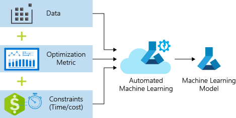
本教程介绍如何通过 Azure 机器学习 Python SDK 使用 Azure 机器学习自动化 ML 训练回归模型。 此回归模型预测纽约出租车费用。
此过程接受定型数据和配置设置,并自动循环访问不同特征规范化/标准化方法、模型和超参数设置的组合,以实现最佳模型。
你将在本教程中使用 Python SDK 编写代码。 你将了解如何执行以下任务:
- 使用 Azure 开放数据集下载、转换和清理数据
- 定型自动化机器学习回归模型
- 计算模型准确度
对于无代码 AutoML,请尝试以下教程:
如果没有 Azure 订阅,请在开始前创建一个试用版订阅。 立即尝试 Azure 机器学习的试用版订阅。
- 如果还没有 Azure 机器学习工作区或计算实例,请完成快速入门:Azure 机器学习入门。
- 完成快速入门后:
- 在工作室中选择“笔记本”。
- 选择“示例”选项卡。
- 打开 tutorials/regression-automl-nyc-taxi-data/regression-automated-ml.ipynb 笔记本。
- 若要运行教程中的每个单元格,请选择“克隆此笔记本”
如果你想要在自己的本地环境中运行此教程,也可以在 GitHub 上找到它。 若要获取所需的包,
- 安装完整的
automl客户端。 - 运行
pip install azureml-opendatasets azureml-widgets以获取所需的包。
导入必需包。 “开放数据集”包内有表示各个数据源的类(如 NycTlcGreen),用于在下载前轻松筛选日期参数。
from azureml.opendatasets import NycTlcGreen
import pandas as pd
from datetime import datetime
from dateutil.relativedelta import relativedelta
首先,创建用于保留出租车数据的数据帧。 如果是在非 Spark 环境中,开放数据集仅允许一次下载一个月的数据,并利用一些类来避免较大数据集出现 MemoryError。
若要下载出租车数据,请以迭代方式一次提取一个月的数据,并在将数据追加到 green_taxi_df 前,先从各月的数据中随机采样 2000 个样本,以免数据帧膨胀。 然后,预览数据。
green_taxi_df = pd.DataFrame([])
start = datetime.strptime("1/1/2015","%m/%d/%Y")
end = datetime.strptime("1/31/2015","%m/%d/%Y")

for sample_month in range(12):
    temp_df_green = NycTlcGreen(start + relativedelta(months=sample_month), end + relativedelta(months=sample_month)) \
        .to_pandas_dataframe()
    green_taxi_df = green_taxi_df.append(temp_df_green.sample(2000))

green_taxi_df.head(10)
| vendorID | lpepPickupDatetime | lpepDropoffDatetime | passengerCount | tripDistance | puLocationId | doLocationId | pickupLongitude | pickupLatitude | dropoffLongitude | ... | paymentType | fareAmount | extra | mtaTax | improvementSurcharge | tipAmount | tollsAmount | ehailFee | totalAmount | tripType |
|---|---|---|---|---|---|---|---|---|---|---|---|---|---|---|---|---|---|---|---|---|
| 131969 | 2 | 2015-01-11 05:34:44 | 2015-01-11 05:45:03 | 3 | 4.84 | 无 | 无 | -73.88 | 40.84 | -73.94 | ... | 2 | 15.00 | 0.50 | 0.50 | 0.3 | 0.00 | 0.00 | nan | 16.30 |
| 1129817 | 2 | 2015-01-20 16:26:29 | 2015-01-20 16:30:26 | 1 | 0.69 | 无 | 无 | -73.96 | 40.81 | -73.96 | ... | 2 | 4.50 | 1.00 | 0.50 | 0.3 | 0.00 | 0.00 | nan | 6.30 |
| 1278620 | 2 | 2015-01-01 05:58:10 | 2015-01-01 06:00:55 | 1 | 0.45 | 无 | 无 | -73.92 | 40.76 | -73.91 | ... | 2 | 4.00 | 0.00 | 0.50 | 0.3 | 0.00 | 0.00 | nan | 4.80 |
| 348430 | 2 | 2015-01-17 02:20:50 | 2015-01-17 02:41:38 | 1 | 0.00 | 无 | 无 | -73.81 | 40.70 | -73.82 | ... | 2 | 12.50 | 0.50 | 0.50 | 0.3 | 0.00 | 0.00 | nan | 13.80 |
| 1269627 | 1 | 2015-01-01 05:04:10 | 2015-01-01 05:06:23 | 1 | 0.50 | 无 | 无 | -73.92 | 40.76 | -73.92 | ... | 2 | 4.00 | 0.50 | 0.50 | 0 | 0.00 | 0.00 | nan | 5.00 |
| 811755 | 1 | 2015-01-04 19:57:51 | 2015-01-04 20:05:45 | 2 | 1.10 | 无 | 无 | -73.96 | 40.72 | -73.95 | ... | 2 | 6.50 | 0.50 | 0.50 | 0.3 | 0.00 | 0.00 | nan | 7.80 |
| 737281 | 1 | 2015-01-03 12:27:31 | 2015-01-03 12:33:52 | 1 | 0.90 | 无 | 无 | -73.88 | 40.76 | -73.87 | ... | 2 | 6.00 | 0.00 | 0.50 | 0.3 | 0.00 | 0.00 | nan | 6.80 |
| 113951 | 1 | 2015-01-09 23:25:51 | 2015-01-09 23:39:52 | 1 | 3.30 | 无 | 无 | -73.96 | 40.72 | -73.91 | ... | 2 | 12.50 | 0.50 | 0.50 | 0.3 | 0.00 | 0.00 | nan | 13.80 |
| 150436 | 2 | 2015-01-11 17:15:14 | 2015-01-11 17:22:57 | 1 | 1.19 | 无 | 无 | -73.94 | 40.71 | -73.95 | ... | 1 | 7.00 | 0.00 | 0.50 | 0.3 | 1.75 | 0.00 | nan | 9.55 |
| 432136 | 2 | 2015-01-22 23:16:33 2015-01-22 23:20:13 1 0.65 | 无 | 无 | -73.94 | 40.71 | -73.94 | ... | 2 | 5.00 | 0.50 | 0.50 | 0.3 | 0.00 | 0.00 | nan | 6.30 |
删除训练或其他特征生成不需要的一些列。 自动化机器学习将自动处理基于时间的特征,例如 lpepPickupDatetime。
columns_to_remove = ["lpepDropoffDatetime", "puLocationId", "doLocationId", "extra", "mtaTax",
                     "improvementSurcharge", "tollsAmount", "ehailFee", "tripType", "rateCodeID",
                     "storeAndFwdFlag", "paymentType", "fareAmount", "tipAmount"
                    ]
for col in columns_to_remove:
    green_taxi_df.pop(col)

green_taxi_df.head(5)
对新数据帧运行 describe() 函数,以查看各个字段的汇总统计信息。
green_taxi_df.describe()
| vendorID | passengerCount | tripDistance | pickupLongitude | pickupLatitude | dropoffLongitude | dropoffLatitude | totalAmount | month_num day_of_month | day_of_week | hour_of_day |
|---|---|---|---|---|---|---|---|---|---|---|
| count | 48000.00 | 48000.00 | 48000.00 | 48000.00 | 48000.00 | 48000.00 | 48000.00 | 48000.00 | 48000.00 | 48000.00 |
| 平均值 | 1.78 | 1.37 | 2.87 | -73.83 | 40.69 | -73.84 | 40.70 | 14.75 | 6.50 | 15.13 |
| std | 0.41 | 1.04 | 2.93 | 2.76 | 1.52 | 2.61 | 1.44 | 12.08 | 3.45 | 8.45 |
| min | 1.00 | 0.00 | 0.00 | -74.66 | 0.00 | -74.66 | 0.00 | -300.00 | 1.00 | 1.00 |
| 25% | 2.00 | 1.00 | 1.06 | -73.96 | 40.70 | -73.97 | 40.70 | 7.80 | 3.75 | 8.00 |
| 50% | 2.00 | 1.00 | 1.90 | -73.94 | 40.75 | -73.94 | 40.75 | 11.30 | 6.50 | 15.00 |
| 75% | 2.00 | 1.00 | 3.60 | -73.92 | 40.80 | -73.91 | 40.79 | 17.80 | 9.25 | 22.00 |
| max | 2.00 | 9.00 | 97.57 | 0.00 | 41.93 | 0.00 | 41.94 | 450.00 | 12.00 | 30.00 |
从汇总统计信息中可以看到,有几个字段包含离群值或会降低模型准确度的值。 首先筛选位于曼哈顿区域边界内的纬度/经度字段。 这会筛选出较长的出租车行程,或者在与其他特征的关系上属于离群值的行程。
此外,筛选大于 0 但小于 31 英里(两个纬度/经度对之间的迭加正弦波距离)的 tripDistance 字段。 这会消除行程费用不一致的长离群行程。
最后,totalAmount 字段包含出租车费的负值,这在我们的模型上下文中没有意义,而 passengerCount 字段包含最小值为 0 的错误数据。
使用查询函数筛选掉这些异常,然后删除定型不需要的最后几列。
final_df = green_taxi_df.query("pickupLatitude>=40.53 and pickupLatitude<=40.88")
final_df = final_df.query("pickupLongitude>=-74.09 and pickupLongitude<=-73.72")
final_df = final_df.query("tripDistance>=0.25 and tripDistance<31")
final_df = final_df.query("passengerCount>0 and totalAmount>0")

columns_to_remove_for_training = ["pickupLongitude", "pickupLatitude", "dropoffLongitude", "dropoffLatitude"]
for col in columns_to_remove_for_training:
    final_df.pop(col)
重新对数据调用 describe(),以确保清理工作符合预期。 至此,已有经过准备和清理的出租车、节假日和天气数据集,用于机器学习模型定型。
final_df.describe()
从现有工作区创建工作区对象。 工作区是可接受 Azure 订阅和资源信息的类。 它还可创建云资源来监视和跟踪模型运行。 Workspace.from_config() 读取文件 config.json 并将身份验证详细信息加载到名为 ws 的对象。 在本教程中,ws 在代码的其余部分使用。
from azureml.core.workspace import Workspace
ws = Workspace.from_config()
使用 scikit-learn 库中的 train_test_split 函数将数据拆分为训练集和测试集。 该函数将数据分成用于模型训练的 x(特征)数据集和用于测试的 y(用于预测的值)数据集。
test_size 参数决定了分配用于测试的数据的百分比。 random_state 参数设置随机生成器的种子。这样一来,训练-测试拆分是有确定性的。
from sklearn.model_selection import train_test_split

x_train, x_test = train_test_split(final_df, test_size=0.2, random_state=223)
此步骤的目的是通过数据点来测试完成的模型(此模型尚未用于训练模型),以便测量实际准确性。
换句话说,经过良好训练的模型应该能够准确地根据其尚未看到的数据进行预测。 现已准备好用于自动训练机器学习模型的数据。
若要自动训练模型,请执行以下步骤:
- 定义试验运行的设置。 将训练数据附加到配置,并修改用于控制训练过程的设置。
- 提交用于模型优化的试验。 在提交试验以后,此过程会根据定义的约束循环访问不同的机器学习算法和超参数设置。 它通过优化准确性指标来选择最佳拟合模型。
定义用于训练的试验参数和模型设置。 查看设置的完整列表。 提交带这些默认设置的试验大约需要 5-20 分钟,但如果需要缩短运行时间,可减小 experiment_timeout_hours 参数。
| 属性 | 本教程中的值 | 说明 |
|---|---|---|
| iteration_timeout_minutes | 10 | 每个迭代的时间限制(分钟)。 对于每次迭代需要更多时间的更大数据集,增加此值。 |
| experiment_timeout_hours | 0.3 | 在试验结束之前,所有合并的迭代所花费的最大时间量(以小时为单位)。 |
| enable_early_stopping | True | 如果分数在短期内没有提高,则进行标记,以提前终止。 |
| primary_metric | spearman_correlation | 要优化的指标。 将根据此指标选择最佳拟合模型。 |
| featurization | auto | 如果使用“auto”,则试验可以预处理输入数据(处理缺失的数据、将文本转换为数字,等等) |
| verbosity | logging.INFO | 控制日志记录的级别。 |
| n_cross_validations | 5 | 在验证数据未指定的情况下,需执行的交叉验证拆分的数目。 |
import logging

automl_settings = {
    "iteration_timeout_minutes": 10,
    "experiment_timeout_hours": 0.3,
    "enable_early_stopping": True,
    "primary_metric": 'spearman_correlation',
    "featurization": 'auto',
    "verbosity": logging.INFO,
    "n_cross_validations": 5
}
使用定义的训练设置作为 AutoMLConfig 对象的 **kwargs 参数。 另请指定训练数据和模型的类型,后者在此示例中为 regression。
from azureml.train.automl import AutoMLConfig

automl_config = AutoMLConfig(task='regression',
                             debug_log='automated_ml_errors.log',
                             training_data=x_train,
                             label_column_name="totalAmount",
                             **automl_settings)
备注
自动机器学习预处理步骤(特征规范化、处理缺失数据,将文本转换为数字等)成为基础模型的一部分。 使用模型进行预测时,训练期间应用的相同预处理步骤将自动应用于输入数据。
在工作区中创建一个试验对象。 试验充当单个作业的容器。 将定义的 automl_config 对象传递至试验,并将输出设置为 True,以便查看作业过程中的进度。
启动试验后,显示的输出会随着试验的运行实时更新。 可以看到每次迭代的模型类型、运行持续时间以及训练准确性。 字段 BEST 根据指标类型跟踪运行情况最好的训练分数。
from azureml.core.experiment import Experiment
experiment = Experiment(ws, "Tutorial-NYCTaxi")
local_run = experiment.submit(automl_config, show_output=True)
Running on local machine
Parent Run ID: AutoML_1766cdf7-56cf-4b28-a340-c4aeee15b12b
Current status: DatasetFeaturization. Beginning to featurize the dataset.
Current status: DatasetEvaluation. Gathering dataset statistics.
Current status: FeaturesGeneration. Generating features for the dataset.
Current status: DatasetFeaturizationCompleted. Completed featurizing the dataset.
Current status: DatasetCrossValidationSplit. Generating individually featurized CV splits.
Current status: ModelSelection. Beginning model selection.

****************************************************************************************************
ITERATION: The iteration being evaluated.
PIPELINE: A summary description of the pipeline being evaluated.
DURATION: Time taken for the current iteration.
METRIC: The result of computing score on the fitted pipeline.
BEST: The best observed score thus far.
****************************************************************************************************

 ITERATION   PIPELINE                                       DURATION      METRIC      BEST
         0   StandardScalerWrapper RandomForest             0:00:16       0.8746    0.8746
         1   MinMaxScaler RandomForest                      0:00:15       0.9468    0.9468
         2   StandardScalerWrapper ExtremeRandomTrees       0:00:09       0.9303    0.9468
         3   StandardScalerWrapper LightGBM                 0:00:10       0.9424    0.9468
         4   RobustScaler DecisionTree                      0:00:09       0.9449    0.9468
         5   StandardScalerWrapper LassoLars                0:00:09       0.9440    0.9468
         6   StandardScalerWrapper LightGBM                 0:00:10       0.9282    0.9468
         7   StandardScalerWrapper RandomForest             0:00:12       0.8946    0.9468
         8   StandardScalerWrapper LassoLars                0:00:16       0.9439    0.9468
         9   MinMaxScaler ExtremeRandomTrees                0:00:35       0.9199    0.9468
        10   RobustScaler ExtremeRandomTrees                0:00:19       0.9411    0.9468
        11   StandardScalerWrapper ExtremeRandomTrees       0:00:13       0.9077    0.9468
        12   StandardScalerWrapper LassoLars                0:00:15       0.9433    0.9468
        13   MinMaxScaler ExtremeRandomTrees                0:00:14       0.9186    0.9468
        14   RobustScaler RandomForest                      0:00:10       0.8810    0.9468
        15   StandardScalerWrapper LassoLars                0:00:55       0.9433    0.9468
        16   StandardScalerWrapper ExtremeRandomTrees       0:00:13       0.9026    0.9468
        17   StandardScalerWrapper RandomForest             0:00:13       0.9140    0.9468
        18   VotingEnsemble                                 0:00:23       0.9471    0.9471
        19   StackEnsemble                                  0:00:27       0.9463    0.9471
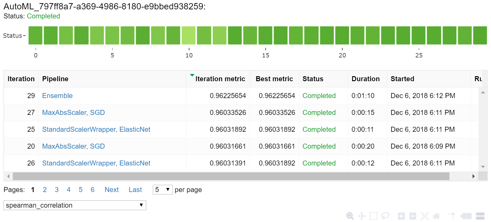
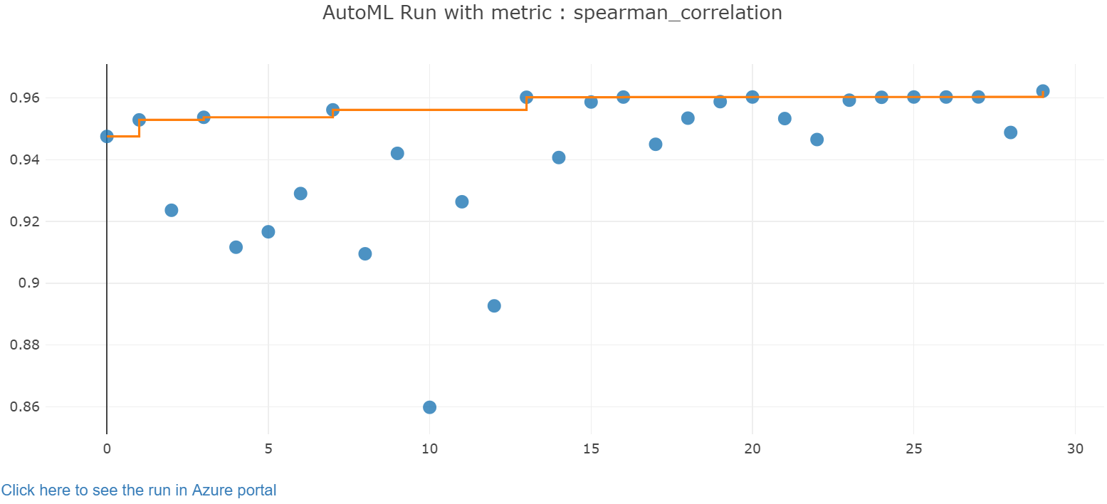
通过 Jupyter 小组件浏览自动训练的结果。 此小组件支持查看每个作业迭代的图和表,以及训练准确度指标和元数据。 此外,可以筛选不同于下拉选择器中的主要指标的准确度指标。
from azureml.widgets import RunDetails
RunDetails(local_run).show()
选择迭代后的最佳模型。 get_output 函数针对上次拟合调用返回最佳运行和拟合的模型。 在 get_output 中使用重载,可以针对任何记录的指标或特定的迭代来检索最佳运行和拟合的模型。
best_run, fitted_model = local_run.get_output()
print(best_run)
print(fitted_model)
使用最佳模型针对测试数据集运行预测,以便预测出租车费。 函数 predict 使用最佳模型根据 x_test 数据集预测 y(行程费用)的值。 输出 y_predict 中头 10 个预测的费用值。
y_test = x_test.pop("totalAmount")

y_predict = fitted_model.predict(x_test)
print(y_predict[:10])
计算结果的 root mean squared error。 将 y_test 数据帧转换为要与预测值比较的列表。 函数 mean_squared_error 接受两个数组的值,计算两个数组之间的平均平方误差。 取结果的平方根会将相同单位的误差提供为 y 差异(成本)。 它大致指出了出租车费预测值与实际费用之间有多大的差距。
from sklearn.metrics import mean_squared_error
from math import sqrt

y_actual = y_test.values.flatten().tolist()
rmse = sqrt(mean_squared_error(y_actual, y_predict))
rmse
运行以下代码,使用完整的 y_actual 和 y_predict 数据集来计算平均绝对百分比误差 (MAPE)。 此指标计算每个预测值和实际值之间的绝对差,将所有差值求和。 然后,它将总和表示为实际值总和的百分比。
sum_actuals = sum_errors = 0

for actual_val, predict_val in zip(y_actual, y_predict):
    abs_error = actual_val - predict_val
    if abs_error < 0:
        abs_error = abs_error * -1

    sum_errors = sum_errors + abs_error
    sum_actuals = sum_actuals + actual_val

mean_abs_percent_error = sum_errors / sum_actuals
print("Model MAPE:")
print(mean_abs_percent_error)
print()
print("Model Accuracy:")
print(1 - mean_abs_percent_error)
Model MAPE:
0.14353867606052823

Model Accuracy:
0.8564613239394718
从两个预测准确度指标来看,该模型可以很好地根据数据集的特征来预测出租车费,误差率大约为 15%,通常在 4.00 美元上下。
传统的机器学习模型开发过程是资源高度密集型的,需要大量的领域知识和时间投资来运行数十个模型并比较其结果。 使用自动化机器学习是一种很好的方式,可以针对方案快速测试许多不同的模型。
如果打算运行其他 Azure 机器学习教程,请不要完成本部分。
如果使用了计算实例,请在不使用 VM 时将其停止,以降低成本。
在工作区中选择“计算”。
从列表中选择计算实例的名称。
选择“停止” 。
准备好再次使用服务器时,选择“启动” 。
如果不打算使用已创建的资源,请删除它们,以免产生任何费用。
- 在 Azure 门户中,选择最左侧的“资源组”。
- 从列表中选择已创建的资源组。
- 选择“删除资源组”。
- 输入资源组名称。 然后选择“删除”。
还可保留资源组,但请删除单个工作区。 显示工作区属性,然后选择“删除”。
在本自动化机器学习教程中,你已完成以下任务:
- 配置了工作区并准备了试验数据。
- 结合自定义参数在本地使用自动化回归模型进行了训练。
- 浏览并查看了训练结果。